Johns Hopkins APL Technical Digest
MLM: Machine Learning for Threat Characterization of Unidentified Metagenomic Reads

Benjamin D. Baugher, Phillip T. Koshute, N. Jordan Jameson, Kennan C. Lejeune, Joseph D. Baugher, and Christopher M. Gifford
Abstract
Forensics and military investigators often assess sites of interest, searching for evidence of biological hazards. The application of metagenomics provides genomic data for all microorganisms present in a sample, enabling advanced analysis for detection of biological signatures and threat detection from such sites. DNA sequence segments (digitally represented as “reads”) from metagenomics samples are commonly compared with reference libraries in order to identify microorganisms present in the sample. However, this approach does not capture the complete biological signature, as there always remains a subset of reads that are unable to be successfully mapped to a known organism. The Johns Hopkins University Applied Physics Laboratory (APL) Machine Learning for Metagenomics (MLM) pipeline characterizes these unidentified reads in terms of composition and alignment with sequences of known organisms. Since these reads are unable to be mapped directly to a known organism, our models classify each read according to one of five threat levels, ranging from 0 to 4 (with threat level 4 the most severe). Our pipeline consists of random forest, Bayesian network, and clustering models. When testing this pipeline against simulated and real sequencing data, we achieved high threat level classification accuracy: 95% for clusters of related reads. Based on these results, we are preparing for deployment of our pipeline on far-forward devices, providing investigators with real-time threat assessment of biological materials to inform an appropriate rapid response.
Download this article or scroll to continue reading
Introduction
Forensics and military investigators often assess sites of interest, searching for evidence of biological hazards due to malicious actors or natural phenomena.1 When hazards are present, it is ideal to identify them precisely. However, if this is not possible, characterizing the severity of the threat provides vital insights for guiding the investigators’ response.
Metagenomics enables detailed screening of biological samples from sites of interest. Collected samples can be passed through a sequencer, yielding reads of DNA nucleotides. A read is a digital representation of a segment of a DNA molecule. In an attempt to identify the organisms present in a sample, the reads are compared with reference libraries of DNA sequences from known organisms. Close matches with reference sequences infer the presence of specific organisms in the sample. However, there always remains a subset of reads that are unable to be successfully mapped to a known organism based on the set of matches, if any, to reference sequences. For instance, emerging, mutated, or modified threats all potentially pose concern to investigators but often do not have matches within reference libraries. Additionally, reference sequences exist only for a small percentage of microorganisms.
Our Machine Learning for Metagenomics (MLM) project focuses on these unmapped reads (i.e., “unidentified” reads). We developed a pipeline of models that characterizes unidentified reads in terms of composition and alignment with sequences of known organisms. Since these reads are unable to be mapped directly to a known organism, our models classify each read according to one of five threat levels (TLs), ranging from 0 to 4. We developed this scale of TLs by combining the bioterrorism categories from the US Centers for Disease Control and Prevention2 and the biosafety risk groups from the US National Institutes of Health.3 Within our scale, organisms that pose the greatest threat have TL4, while organisms that do not pose a threat have TL0. By predicting the TL of the organism(s) represented by unidentified reads through carefully trained classification models, MLM provides rapid TL assessments of unidentified organisms present in biological samples (e.g., organisms that are unknown or are not represented within a reference library). We focus specifically on detecting bacterial and viral threats because they comprise the large majority of organisms that pose threats to human health.
The remainder of this article proceeds as follows. We first give a detailed overview of the components of our MLM model pipeline. Then, we describe how we trained the models within the pipeline, enabling the models’ training algorithms to search for patterns between reads with the same TLs. Next, we highlight the pipeline’s results on both simulated and real reads and offer observations on practical considerations for deploying our pipeline. Finally, we suggest possible next steps for ongoing and future research.
Model Setup
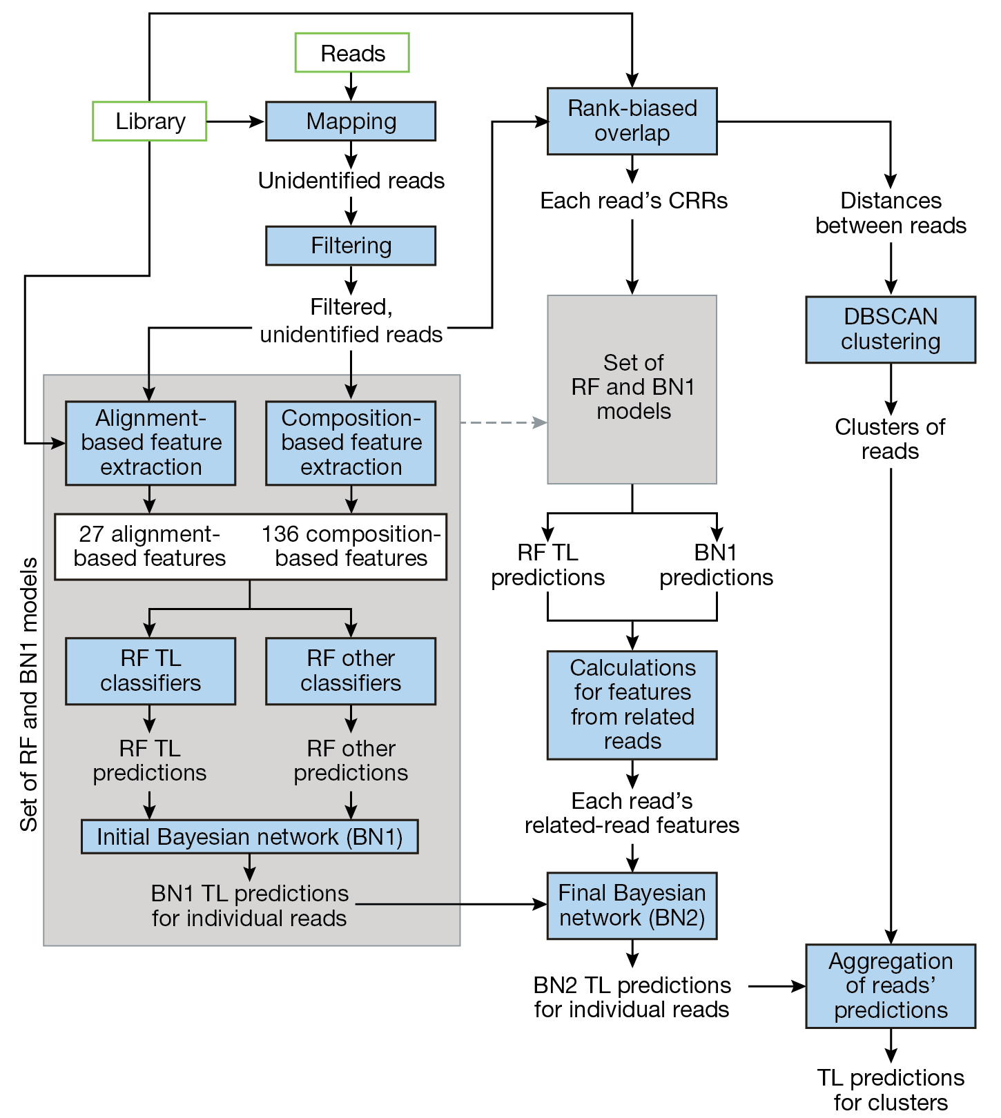
Our MLM pipeline consists of interconnected processing steps, random forest (RF) models, Bayesian network (BN) models, and clustering steps. Figure 1 illustrates the progression of reads through these steps and models. Within the pipeline, unidentified reads are gathered and filtered, features are extracted from remaining reads, and these features are passed through a combination of models. The ensemble of RF models provides preliminary prediction of the TLs of the unidentified organisms represented by the reads and of other characteristics. The initial BN (BN1) fuses the RF predictions. The final BN (BN2) incorporates features computed from the predictions of each individual read’s closely related reads (CRRs). The clustering step is based on the density-based spatial clustering for applications with noise (DBSCAN) method and enables a single aggregate TL prediction for the organisms represented in each cluster. Each of these steps is further described in the following subsections.
Figure 1
Data flow through model pipeline. Unidentified reads are gathered and filtered, features are extracted from remaining reads, and these features are passed through a combination of models. The ensemble of RF models provides preliminary prediction of the TLs of the reads’ organisms, as well as other characteristics. The initial BN (BN1) fuses the RF predictions. The final BN (BN2) incorporates features computed from the predictions of each individual read’s closely related reads (CRRs). The clustering step is based on the density-based spatial clustering for applications with noise (DBSCAN) method and enables a single aggregate TL prediction for the organisms represented in each cluster of reads.
Read Source
Among the multitude of available sequencing devices, we focus our analysis on sequencing data from the Oxford Nanopore MinION sequencer.4 We opted for the MinION device because of its portability, low cost, and ease of use—characteristics that are important in many use cases for military investigators. All of the reads within this analysis have either come from a MinION simulator (refer to the Read Simulation subsection) or have been collected with a MinION device or similar nanopore sequencing device (refer to the Results on Real Reads subsection).
If desired, our process for extracting features and developing and evaluating models could be similarly implemented for reads from other sequencing platforms for which data are available. For instance, we have previously demonstrated this capability for Illumina’s MiSeq and iSeq platforms.
Read Mapping with Reference Library
Before mapping, we pass reads through an algorithm that flags reads that are highly likely to originate from macroorganism (host organism) contamination. This algorithm searches for matches in a set of short overlapping k-mers between the read and a database of plant and animal reference sequences that are extremely unlikely to have occurred by chance. (A k-mer is a subsequence of nucleotides of length k.) We discard reads that correspond to such matches.
To identify remaining reads that can be mapped to known microorganisms, we developed a pair of matching and alignment algorithms. Relying on clever indexing of large reference libraries and overlapping short k-mer matches, the first algorithm is very fast but at the cost of some accuracy. The second algorithm verifies matches identified by the first algorithm by performing targeted alignments between a given read and the portion of the reference sequence in which the potential match was found.
The matching algorithm yields an alignment score between each read and the top N reference sequence matches, where N is a user-defined parameter. Ultimately, an alignment hit occurs when the alignment score between the read and a reference sequence exceeds a specified threshold. This alignment score is also used for feature extraction in the cases where the scores do not exceed the threshold (refer to the Feature Extraction subsection).
Currently, we use as our reference library the October 2, 2021, version of the Nucleotide database from the National Center for Biotechnology Information.5 We plan to update our reference library periodically as we move forward with this project.
After this matching step, we annotate reads for which we have identified alignment hits with known organisms and provide them to the end user for analysis. The remaining reads without alignment hits (i.e., unmapped reads) are then processed by our MLM pipeline to search for any undetected threats from emerging, mutated, or modified microorganisms. By assessing the unmapped reads, our MLM pipeline aims to complement the insights obtained from reads mapped to known organisms. The MLM pipeline can also be used to assess the unidentified reads from any other alignment or taxonomic classifier tool.
Filtering Unidentified Reads
To select the best set of reads from a given sample to run through our model pipeline, we employ a variety of filtering steps.
First, we check the number of nucleotides that are suitable for assessment. After masking likely MinION sequencing adapters6 and low complexity regions,7 we discard reads that do not have at least 100 unmasked nucleotides.
We also consider the quality scores of each read, checking whether a read has enough high-quality nucleotides and a sufficiently long sequence of contiguous high-quality nucleotides. We discard reads that do not meet both of these conditions.
Each of the filtering steps is based on parameters that can be tuned to be more or less aggressive based on the use case and end user needs. Our default parameter values are somewhat conservative, yielding greater confidence in the results. In contrast, a more liberal approach would enable greater sensitivity to traces of potential threats, but at the cost of an increased false alarm rate (FAR). A false alarm (FA) occurs when the MLM pipeline predicts a high TL but the true TL is not high. We regard TL2, TL3, and TL4 as high TLs.
Feature Extraction
For all unidentified reads remaining after filtering, we extract 163 features, including 19 alignment-based features and 144 composition-based features. These features are ultimately used as inputs to six subsequent RF models.
We obtain the alignment-based features by comparing each read with sequences of reference organisms for which we know the TL. These alignment-based features include the TL of the reference sequence most closely aligned to the read under consideration, the top alignment scores for reference sequences from each TL (i.e., one feature for each of the five TLs), and the percentage of alignment hits from each TL.
While alignment-based features seek to quantify and represent a read’s similarities to known organisms, composition-based features focus directly on the nucleotides that make up a given read. Most of the composition-based features correspond to the frequencies of the 136 unique tetramers. Other composition-based features include the GC (guanine-cytosine) content of the read and minimum compositional distances to reference sequences from each TL.
Taken together, the alignment- and composition-based features provide a detailed representation of each read. Subsequent supervised machine learning (ML) models leverage this representation to find patterns between reads’ features and the TLs of the organisms from which they have come.
Random Forest Classifiers
RF models are supervised ML models consisting of numerous decision trees, each trained by a statistically strategic random subset of the available data.8 The random selection of each tree’s training data reduces the correlation in the trees’ prediction, amounting to less prediction variance and less overall prediction error for the RF. Within the RF, each decision tree yields a separate prediction based on a set of logical rules, which can be evaluated by progressing down the tree. For our data, examples of such logical rules might include “top normalized alignment score for a TL3 reference sequence < 0.4” or “normalized frequency of tetramer #1 > 0.05.”
Our MLM pipeline includes six RF classification models (or “classifiers”). Four of the RF classifiers predict TLs. Each of these TL classifiers is trained with a different set of simulated reads. (We describe our simulation process in the Read Simulation subsection.) Each set is characterized by whether its reads originated from a bacterium or virus and which clade (species or strain) of “neighbors” has been removed from the reference library before those reads’ features have been computed. We remove the neighbor clade as a way to mimic the scenario in which a read from a previously unseen species or strain is collected. We refer to the RF TL classifiers according to the set of reads on which they were trained: BSp (bacteria reads with their species removed from the reference library), BStr (bacteria reads with their strains removed from reference library), VSp (virus reads with their species removed from the reference library), and VStr (virus reads with their strains removed from reference library). We train separate RF classifiers for each set of reads to cover a range of possible unidentified organisms from which reads might be collected. The predictions from these RFs are ultimately fused (along with other values) by the BNs later in the pipeline.
The other two RF classification models predict other characteristics of the reads. The BV classifier predicts whether a given read corresponds to bacterium or virus. Likewise, the NN classifier predicts whether the closest related organism in the reference library is in the same species or not (“nearest neighbor”). The outputs of these additional RF classifiers also are inputs to the BNs within the MLM pipeline.
Initial Bayesian Network
BNs represent probability relationships between variables, enabling the state of one or more variables to be assessed as data are observed. In particular, BNs provide an estimate of the “belief level” for each possible state of each variable, based on prior knowledge of these variables and observed data.
In a BN, each variable is defined by a node, which has two or more possible discrete states. The “target” node has special importance; this node represents the variable for which the state is being estimated. Pairs of nodes with conditional probability relationships have a directed edge between them; the edge originates at the node corresponding to the variable on which the other variable is conditioned. A node may be the terminus for more than one directed edge (i.e., a variable may be conditioned on more than one other variable).
The structure of a BN’s nodes and edges may be determined through expert knowledge or “learned” via training data. We determined through experimentation that learning the BN structure yields better prediction performance. Our approach for training our BNs is described in the Model Training Details subsection.
Each node also has a conditional probability table (CPT), which describes the conditional probability relationships between nodes connected by edges. The dimension of each node’s CPT is determined by the number of variables on which the variable corresponding to that node is conditioned. In general, the values in each column of a CPT sum to 1.
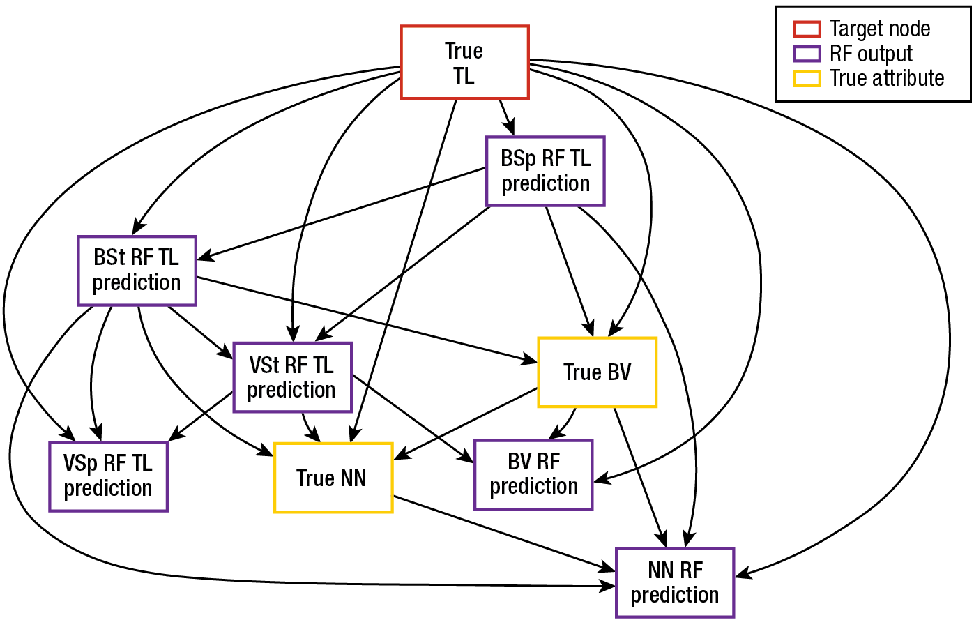
BN1 includes nodes for nine variables: the outputs of the six RF classifiers, the true type of read (bacterium or virus), the true removed clade (species or strain), and the read’s TL (i.e., TL of the organism from which the read has come). For each read, we compute values for the first six variables. When these values are propagated through BN1, the BN1 inference step estimates values for the remaining three variables, including the read’s TL. Figure 2 gives an example of a possible structure for BN1. Based on this particular BN1 structure, Table 1 gives an example of a CPT for one of the nodes (BSp RF TL Prediction).
The output of the BN is a set of belief values for each node, with one belief value for each state of the variable represented by that node. The belief values range from 0 to 1 and must sum to 1 for a given node. (In Table 1, the sum of each column may slightly differ from 1 because of rounding.) For BN1, these values can be used to predict a discrete TL by identifying the state in the target variable’s node (“Threat Level”) with the largest belief value.
Figure 2
Example of BN1 with learned structure. Included are nodes for nine variables: the outputs of the six RF classifiers, the true type of read (bacterium or virus), the true removed clade (species or strain), and the TL.
| Table 1. Example of BN1 CPT | |||||
| BSp RF TL Prediction | True TL | ||||
| 0 | 1 | 2 | 3 | 4 | |
| 0 | 0.9442 | 0.5895 | 0.1863 | 0.3639 | 0.8501 |
| 1 | 0.0185 | 0.3672 | 0.0351 | 0.5391 | 0.0954 |
| 2 | 0.0018 | 0.0379 | 0.6970 | 0.0280 | 0.0348 |
| 3 | 0.0277 | 0.0046 | 0.0001 | 0.0665 | 0.0003 |
| 4 | 0.0077 | 0.0008 | 0.0816 | 0.0023 | 0.0194 |
| Rows correspond to TLs predicted by the BSp RF model for each read, and columns correspond to the true TL of the organism that each read represents. Each cell shows the probability of the TL predicted by the BSp RF (indicated by the row), given the true TL (indicated by the column). Hence, the values within a given column sum to 1. | |||||
Identifying Closely Related Reads
Within metagenomic analysis, reads are not collected in isolation but rather in samples with sets of thousands to millions of other reads from many different organisms. These sets generally include multiple reads obtained from each organism present. To predict the TL for an individual read, we use features from the read itself as well as from other CRRs that are likely to have come from the same organism or a very closely related one. This mix of features helps us to fine-tune our threat assessment for each read and ultimately reduce FA assessments. Our methods for computing features based on CRRs is described in the Features Based on Closely Related Reads subsection. The model for which these features are inputs is described in the Final Bayesian Network subsection.
To determine the CRRs for each read, we use a method based on rank-biased overlap (RBO).9 For each read, we use segments within the read to match the read with sequences from our reference library. For the reference sequences that match, we align the reads with targeted portions within the reference sequences based on where the segments matched to obtain alignment scores characterizing how well the reads match the reference sequences. These alignment scores are used to produce a ranked list of similar organisms for each read. The list consists of the reference library organisms with the best alignment scores. We repeat this process, obtaining rankings or reference library organisms for each unidentified read. Given these rankings, we compute “distances” between pairs of unidentified reads by comparing the reads’ lists using the RBO method. These distances do not correspond to physical space but instead measure the dissimilarity between reads; reads with similar lists have smaller distances. Originally developed for comparing results of internet search engines, the RBO method enables comparison of ranked and possibly incomplete lists to identify similarities between lists.
For each read, we identify up to 1,000 CRRs from among those with the smallest distances to the read. Not all reads have the full set of 1,000 CRRs. This occurs when there are a limited number of reads present from a given organism. It can also occur with reads that have fewer matches with the reference library. Some reads may even have no CRRs.
Features Based on Closely Related Reads
Given each read’s CRRs, we compute 13 additional features for use as inputs for BN2. These features characterize the predictions of the RF TL classifiers and BN1 for the neighbor reads. Table 2 summarizes these additional features. If a read has no CRRs, CRR_BN1_TLPred_Mode and CRR_BN1_TLPred_Max are set to the BN1 prediction for that read. Likewise, CRR_RF_TLPred_Mode is set to the most common prediction from the RF TL classifiers. All other CRR-related features are set to 0.
BNs expect features with discrete states. Thus, a discrete value must be set for each feature, and special care is needed when there are ties for TL-based features. For the CRR_RF_TLPred_Mode and CRR_BN1_TLPred_Mode features, ties are handled by computing the mean value among all TLs involved in the tie and rounding to the nearest TL. A tie may occur for a given read if multiple TLs are predicted equally often by the CRRs for that read.
Final Bayesian Network
BN2 is similar to BN1 but leverages information from CRRs and incorporates additional features. BN2 involves the 9 nodes from BN1, as well as nodes for the 13 features from Table 2. Similar to BN1, the output of BN2 is a predicted TL for the given read, determined from the TL with the largest belief value in the target node (“Threat Level”).
| Table 2. Summary of neighbor-based features for BN2 | ||
| Feature | Description | Possible Values |
| CRR_RF_TLPred_Mode | The most common output for all RF TL classifiers for all CRRs | 0, 1, 2, 3, 4 |
CRR_RF_PredLevel_TL0 CRR_RF_PredLevel_TL1 CRR_RF_PredLevel_TL2 CRR_RF_PredLevel_TL3 CRR_RF_PredLevel_TL4 | Discrete categories of the proportion p of the RF TL predictions for CRRs with a given TL (the feature value is Low if p < 0.2 for that TL, medium if 0.2 ≤ p < 0.5, and high if p ≥ 0.5) | Low, medium, high |
| CRR_BN1_TLPred_Mode | The most common BN output for CRRs | 0, 1, 2, 3, 4 |
| CRR_BN1_TLPred_Max | The highest TL among BN1 outputs of all CRRs | 0, 1, 2, 3, 4 |
CRR_BN1_PredLevel_TL0 CRR_BN1_PredLevel_TL1 CRR_BN1_PredLevel_TL2 CRR_BN1_PredLevel_TL3 CRR_BN1_PredLevel_TL4 | Discrete categories of the proportion p of the BN1 predictions for CRRs with a given TL (the feature value is low if p < 0.2 for that TL, medium if 0.2 ≤ p < 0.5, and high if p ≥ 0.5) | Low, medium, high |
Clustering
The unidentified reads within our pipeline are composed of very noisy data with a variety of limitations, such as low quality. There are also errors in the reference library. Additionally, reads from low-threat organisms that are somewhat closely related to high-threat organisms may be assessed as posing higher threat than is warranted because of shared genomic regions. As a result, TLs may be incorrectly predicted for individual reads.
To provide a robust alternative to predictions for individual reads, we group the reads within a sample into clusters using the DBSCAN method.10 For each resulting cluster, we obtain cluster-level TL predictions by identifying the most commonly predicted TL for individual reads within the cluster.
The DBSCAN method uses high- and low-density data regions to identify clusters and outliers, characterizing density in terms of reads’ distances from each other. We compute distances between reads as part of the RBO-based CRR identification step (refer to the Identifying Closely Related Reads subsection).
DBSCAN involves two parameters that generally guide the size and number of clusters. The assignment of points to clusters is determined by whether they are in the “neighborhood” of one or more core points. (For our analysis, each read corresponds to a point.) The eps parameter defines the radius of each point’s neighborhood. It can be set as any positive number. Larger values of eps permit more points to be included in a single neighborhood, thus prompting more points to be clustered together and encouraging smaller numbers of clusters. We typically use eps = 0.1. Secondly, the minPts parameter sets the minimum number of other points within a given point’s neighborhood to qualify that point as a “core point.” A point is within another point’s neighborhood if the distance between the points is less than eps. As a result, larger values of minPts make the requirements for a core point to be regarded as a core point more strict and therein also encourage smaller numbers of clusters. Wanting to encourage detection of smaller clusters, we typically set minPts as the minimum of 100 and 0.05NP, where NP is the number of points in a given sample.
Within DBSCAN, points that are not within the neighborhood of any core point are assigned to a “noise cluster.” The points in this cluster are not necessarily similar to each other, but rather are relatively unlike other points assigned to other clusters. Smaller values of eps and larger values of numPts promote more points to be assigned to the noise cluster. In our case, the noise cluster most likely includes reads from contaminating organisms.
Model Training
We train and evaluate models using simulated reads, which provide the benefit of knowing the TLs of the organisms from which they have come. We use the DeepSimulator tool to simulate reads. We split the training reads into multiple sets to separately train the RF models, BN1, and BN2. The following subsections describe our training process in further detail.
Read Simulation
DeepSimulator11,12 is the first deep learning–based MinION read simulator. It seeks to accurately simulate the reads by simulating the entire sequencing process. DeepSimulator directly models the raw electrical signals produced by nanopores, rather than simply trying to mimic the sequencing results. In particular, it builds a context-independent pore model using deep learning methods to simulate the electrical signals produced by the actual nanopores. Given these signals, it uses standard base-calling software to convert the simulated signals into reads.
To train and evaluate the version of our pipeline shown in this analysis, we ran DeepSimulator version 1.5 on selected reference sequences from the Nucleotide database, using the built-in error profile for the MinION sequencer. Additionally, we specified a mean read length of 8,000 nucleotides, a read coverage of 50× for bacterial genomes, and a read coverage of 250× for viral genomes. Read coverage refers to the average number of simulated reads in which a given nucleotide is included. These runs ultimately yielded approximately 372 million simulated reads for bacteria and approximately 70 million reads for viruses.
Simulating Unidentified Reads
To train models to make accurate predictions about unidentified organisms, we construct simulated datasets of “unknown” organisms by removing known organisms from the reference databases (i.e., “sanitizing” the databases). To do this, we remove each clade one by one, compute the features on the simulated reads obtained from the organisms within the removed clade, and then put it back before removing the next clade. For both bacteria and viruses, we construct two datasets apiece. The first one set mimics the case in which an entire new species is encountered without being represented in the reference library. The second set similarly mimics the case in which a new strain is encountered.
We use our read mapping algorithm (refer to the Read Mapping with Reference Library subsection) to classify and then align each of the simulated reads with the sanitized reference database. We discard reads that align well to any reference sequence that remains in the database because these would not be considered to be unidentified reads. The remaining reads are those that would be unidentified if the given clade was in fact unknown; we use these reads for training and testing our models. We set the threshold for regarding a read as unidentified to a 90% alignment match.
Defining Training and Test Sets
We gathered slightly more than 1.4 million unidentified reads from the simulated data described above. We set aside ~25% for testing and separated the rest into different training sets: 136,446 reads for BSp RF; 84,056 for BSt RF; 52,138 for VSp RF; 15,419 for VSt RF; 284,925 for BN1; and 490,522 for BN2. The different types of reads used to train our four TL RF classifiers are described in the Feature Extraction subsection. We formed an additional training set as the union of the four training sets for RF TL classifiers (amounting to 288,059 reads) and used this aggregate set to train both the BV and NN RF classifiers.
For each training set we extract 163 features from each read within the set (refer to the Feature Extraction subsection). Training ML models involves allowing computerized algorithms to find patterns that link input features to the target value. We train six RF models using the feature data extracted from their individual training sets. As described in the Random Forest Classifiers subsection, the first four RF models predict the read’s TL; these models differ in the type of reads used to train them (BSp, BSt, VSp, VSt). The other two RF models predict whether the read is from a bacterium or virus for the BV classifier and whether the closest related organism in the reference library is in the same species or not for the NN classifier. Subsequently we run the feature data extracted from the BN1 training set through the trained RF models and use the outputs of these models to train BN1 to predict TL. As a final training step, we run the feature data from the BN2 training set through the trained RF and BN1 models, compute CRR-based features (summarized in Table 2), and use the resulting 19 features to train BN2 to predict TL for individual reads (refer to the Final Bayesian Network subsection).
To assess performance, we ran the 346,373 reads from the test set through the entire MLM pipeline. Because these reads were not at all involved in model training, the pipeline’s performance against them provides an estimate of the pipeline’s performance against unidentified threats. The pipeline’s performance against these reads is described in the Results on Simulated Reads subsection.
Model Training Details
We use various R packages to train our models: ranger for the RF models13 and both bnlearn14 and gRain15 for BN1 and BN2.
For the RF models, we use 50 trees per model and ranger default values for all other settings. The minimum number of reads at a terminal node in each decision tree is one, and trees are set to grow as large as the data permit. For each tree, reads are randomly sampled with replacement (i.e., reads can be sampled more than once for a given tree). Each split within each tree considers a subset of 12 randomly selected features (equal to the floor of the square root of the total number of features, floor (√163) ≈ 12).
For training the BN models, we use the hill-climbing algorithm from the hc function within the bnlearn package to learn the structure of the models. To aid the learning, we specify an initial network (with edges originating from the “Threat Level” node and terminating at each of the other nodes) and a list of forbidden edges (e.g., those that terminate at the “Threat Level” node). For BN2, we also limit the number of edges terminating any given node to 3. This constraint limits the size of any given node’s CPT and also decreases the time required to run the model. Likewise, we use the extractCPT, compileCPT, and grain functions within the gRain package to fit the nodes’ CPTs. To account for the possibility in which a given cell in the CPT has zero instances, we specify a smoothing constant of 0.01.
Supporting Evidence Check for False Alarm Reduction
During model development, we observed that FAs occurred because in certain cases reads from the training set with true high TL did not have any supporting evidence for the high TL (i.e., the extracted RF features corresponding to high TLs had low values, suggesting that there were no similarities to high-threat organisms for these reads). As a result, the BN models had learned to associate features that did not reflect similarities to high-threat organisms with high TL predictions. This aspect of the models can lead to FAs because these associations do not generalize well. While there are reads from true high-threat organisms for which we do not find any similarities to known threats, we generally have low confidence in any high TL predictions for which such similarities have not been found.
To account for this phenomenon, we implemented a postprocessing step after BN2 to adjust predicted TLs for which there was no supporting evidence. In particular, if a predicted high TL is not consistent with RF feature values corresponding to that TL, we adjust the belief values for that TL so that it is no higher than any belief value for a low TL and renormalize all TLs’ belief values so that they sum to one. We repeat this step until the highest belief value for the read is for a low TL or for a high TL with supporting evidence. This step substantially reduces the MLM pipeline’s FAR without impacting cluster-level TL predictions for real reads (refer to the Results on Real Reads subsection).
Results
To assess the performance of the MLM pipeline, we evaluated it on both simulated and real reads. For simulated reads, the true TL of the organism from which each read has come is known. The real reads come from collected samples for which the primary organisms present are known. Thus, the true TL for each organism within a set of real reads is known, but the true TLs for individual reads are not necessarily known.
Results on Simulated Reads
As described in the Read Simulation subsection, we simulated reads using the DeepSimulator tool. To account for the randomness in how RF classifiers are constructed, we trained 10 sets of models, tracking results for the test set reads (refer to the Defining Training and Test Sets subsection) on each set of models. We measure performance in terms of accuracy (the proportion of correctly predicted TLs across all reads), sensitivity (the proportion of reads with true high TL for which we predict high TL), and positive predictive value (PPV, the proportion of reads for which we predict high TL that have a true high TL). In other contexts, sensitivity and PPV are also called recall and precision, respectively.
Because the simulated reads are not grouped into samples, we analyzed these metrics at the read level. We did not conduct the clustering step as part of our analysis of simulated reads. While operational decisions are unlikely to be made in practice on individual reads, different models’ PPV and sensitivity on these reads characterize the models’ relative performance and point to which model is most promising for use with clusters of reads.
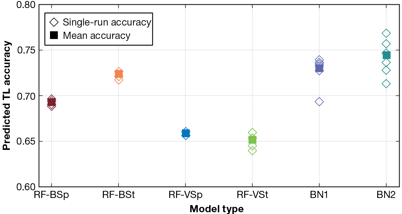
Figure 3 shows the accuracy results for each model type within our pipeline for each set of models. These models undertake the five-class classification problem of predicting a TL for each read from among one of five possible TLs. Incorporating the outputs of the RF models (Figure 1), the BN models perform better than the RF TL classifiers, consistently achieving classification accuracy among the five TLs of 70% or greater and averaging near 75% accuracy. Since the BN models leverage the predictions of the RF TL classifiers, the improved performance with the BN models is expected.
Figure 3
TL classification accuracy (out of five TLs) by model type. The BN models perform better than the RF TL classifiers, consistently achieving 70% or greater classification accuracy and averaging near 75% accuracy.
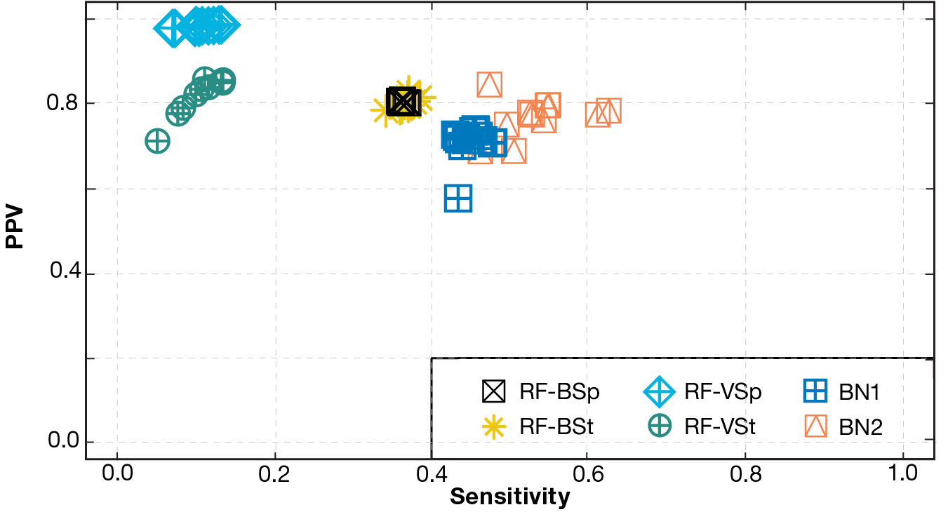
We also assessed the models’ ability to accurately predict high TLs, i.e., to predict whether or not a read has come from an organism with a TL of 2 or higher. Since this amounts to a binary classification problem, the model’s prediction is determined by comparing its output score (i.e., sum of belief values for TL2, TL3, and TL4) with the decision threshold. It is important for models to not miss true TLs (i.e., achieve high sensitivity) and also to not falsely predict high TLs (i.e., achieve high PPV). Figure 4 shows the trade-off between sensitivity and PPV for each model with a decision threshold of 0.5. Again, BN2 showed the best results, with relatively high PPV and moderate sensitivity. Other models, including RF-VSp, showed higher PPV but very low sensitivity.
Figure 4
Trade-off between sensitivity and PPV by model type (with five original TLs consolidated to two low and high TLs). BN2 performed best, with relatively high sensitivity and moderate PPV. Other models showed higher PPV but very low sensitivity.
For some operational decisions, these values (PPV ~0.8, sensitivity ~0.5) may be unsatisfactory. Nevertheless, given the 3-to-1 class imbalance within our test set (with more low TLs than high TLs), they still point to the potential of BN2 to efficiently detect high-TL organisms. Refer to the Results on Real Reads subsection for details on how these read-level performance values translate to success on clusters of reads.
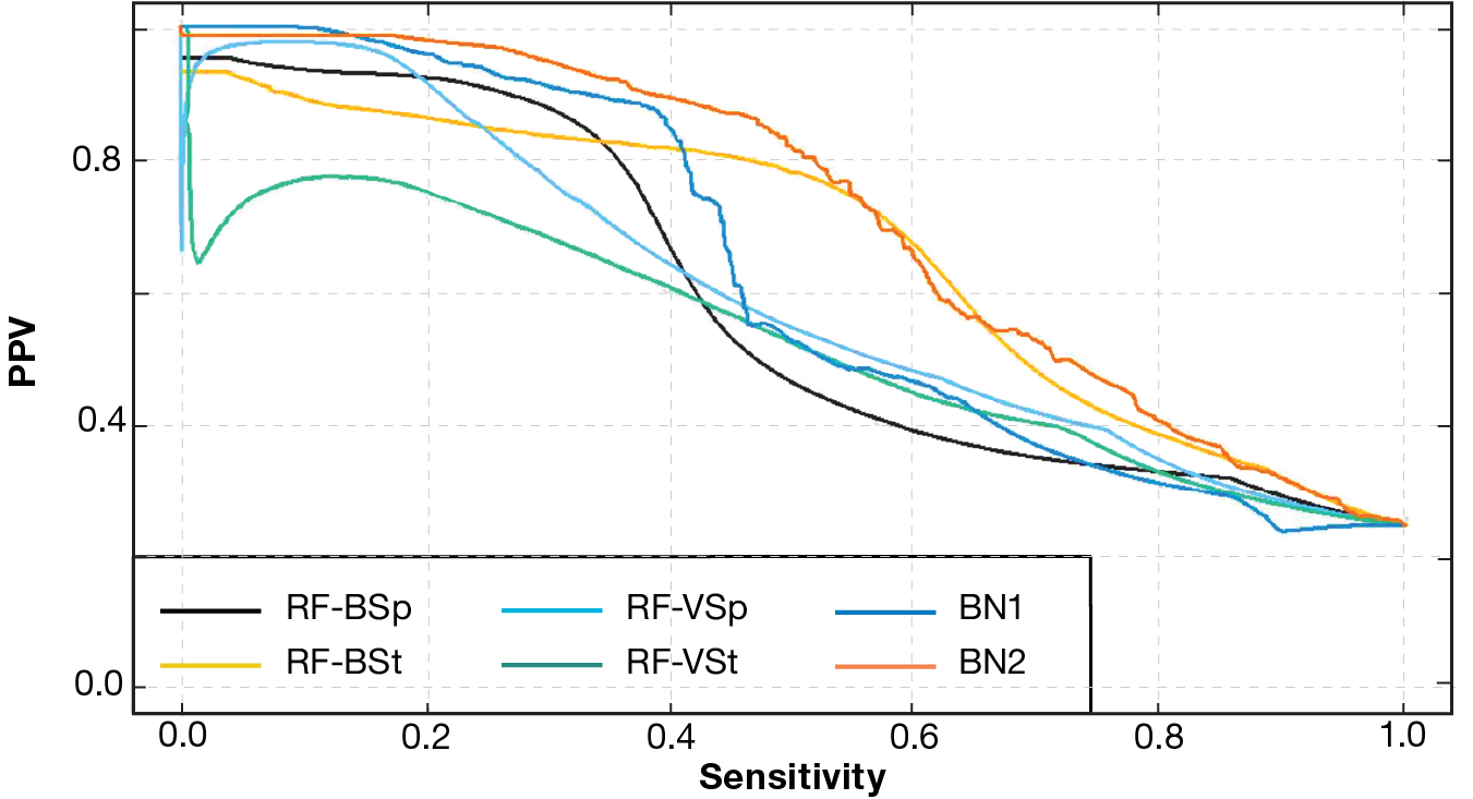
In Figure 5, each model’s PPV-sensitivity curve (also known as a precision-recall curve) shows the values of PPV and sensitivity as the decision threshold is varied. These curves are constructed by aggregating the results from all 10 sets of models. BN2 and RF-BSt show the best performance.
Figure 5
PPV-sensitivity curves (precision-recall curves) by model type. BN2 again performed best. The RF-BSt model also shows good performance.
Results on Real Reads
We also assessed the MLM pipeline using 21 samples of real reads that were prepared, sequenced, and analyzed by an external organization. The samples were analyzed using a bioinformatics pipeline based on minimap2,16 and the unidentified reads were given to us for analysis. We ran each sample through the MLM pipeline (Figure 1). The number of unidentified reads ranged between thousands and hundreds of thousands per sample, and we first ran these through our filters (refer to the Filtering Unidentified Reads subsection). After filtering, the number of reads remaining for analysis from each sample ranged from several dozen to several hundreds of thousands.
From each sample, we applied DBSCAN clustering (refer to the Clustering subsection) and predicted TLs at the cluster level. Accordingly, we evaluated our predictions at the cluster level, comparing the true TL of the highest threat organism (i.e., the true highest TL) with the highest TL predicted for any cluster within the sample. Table 3 shows this comparison, with nonzero counts shown in boldface and underlined for easy reference.
| Table 3. Confusion matrix of TL predictions by real read sample | |||||
| Highest Predicted TL | True Highest TL for Sample | ||||
| 0 | 1 | 2 | 3 | 4 | |
| 0 | 5 | 1 | 0 | 0 | 0 |
| 1 | 0 | 7 | 0 | 0 | 0 |
| 2 | 0 | 0 | 0 | 0 | 0 |
| 3 | 0 | 0 | 0 | 2 | 0 |
| 4 | 0 | 0 | 0 | 0 | 6 |
| Nonzero counts are shown in boldface and underlined. | |||||
We correctly predicted the highest TL for 20 of 21 samples (95%). These results include correct predictions for 8 of 8 samples with TLs of 2 or higher. The one misclassified sample could arguably have been counted as correct as it contained a TL1 organism but only at a very low abundance (0.01%). Based on this abundance level, the expected number of reads present would be well below the MLM pipeline’s specified level of detection. For a given sample, the level of detection is determined by the minimum cluster size (refer to the Clustering subsection). For this sample, the minimum cluster size and level of detection would be 100 reads (i.e., 0.06% of this sample).
We also achieved low FAR against these samples. We did not predict a high TL (TL2 or above) for any of the 13 samples with true low TLs (TL0 or TL1). Thus, our FAR for these cluster-level predictions was 0%. Moreover, for the ~1 million reads within these samples, we had a 0.01% read-level FAR.
Deployment Considerations
Based on the results of the MLM pipeline on both simulated reads and collected samples, we are considering requirements for deployment, including physical size, cost, adaptability, runtime, and interpretability.
Requirements for size, weight, and power depend on whether our model pipeline is run at a nearby mobile laboratory as part of a follow-up analysis or in the field amid a real-time investigation. If the models are run in a laboratory, minimizing size, weight, and power needs is less crucial. Conversely, if the models are run in the field, they must be able to be implemented on devices carried during military missions and other investigations.
For the scenario in which our pipeline is run in the field, the computational requirements must not result in the need for a device that is overly heavy or that requires additional batteries. We are mindful of these constraints, and have selected more efficient design options whenever possible, and made numerous improvements to reduce the memory footprint and runtime of the pipeline. Some examples include a fourfold reduction of our overall memory footprint by implementing a database decimation technique developed for plagiarism detection; an analysis of the effect of the number of trees in our RF models that resulted in substantially smaller models, improving both memory use and runtime; and a redesign of our BN inference implementation that reduced the inference runtime by three orders of magnitude.
The devices must also have a low enough cost and size that they can be feasibly included within an investigator’s tools. In its current setup, the MLM pipeline can run smoothly on a laptop or a miniature personal computer (mini-PC). For instance, we demonstrated that the MLM pipeline can run on a mini-PC (connected wirelessly to the sequencing device) that has a footprint of 20 in.2, weighs 1 lb., and draws only 6 W of power. We also developed a user-friendly web application to enable follow-up analysis on a laptop when desired.
New threats are prone to emerge at any time, and the reference library leveraged by our pipeline may fall out of date. Nevertheless, insofar as we target reads that are not mapped to reference organisms, our approach is robust to intervals without library updates. Moreover, we are able to update the reference library whenever new information becomes available, enabling the models to be retrained if time permits. Several weeks are typically required to fully train and validate the models.
Some investigators may need insights within short time frames to inform their decisions. Thus, we aim for our models to have efficient runtime. The current pipeline can process and analyze approximately 3,200 unidentified reads per minute on a laptop and approximately 1,800 unidentified reads per minute on the mini-PC. For context, MinION sequencers yield about 20,000 reads per hour. Our pipeline does not fully process all of these reads but only those that are unidentified. Although the percentage of unidentified reads can vary considerably between samples, on average the pipeline can process an hour’s worth of sequencing data in approximately one minute on a laptop and in less than two minutes on a mini-PC.
Decision support insights are also enhanced by complementing TL predictions with explanations of how the predictions are determined. To achieve this, we incorporated SHAP (SHapley Additive exPlanations) into our pipeline, which is a popular ML technique for explaining the particular influence that values of individual features have had on the overall TL predictions.17,18 These explanations provide additional information to support decision-making and to increase user confidence in the models.
Possible Next Steps
The models within our MLM pipeline show promising performance, achieving over 74% accuracy in TL classification of individual simulated reads and 95% accuracy for predicting the highest TL present in real samples based on clusters of related reads (refer to the Results section). At the same time, work for this project is ongoing, and several additional capabilities or analyses are underway or planned. These next steps focus on possible new features for the RF models, new features for BN2, and possible alternatives to BN2. Complementing the deployment considerations described in the preceding section, these steps are aimed at further improving the accuracy of the pipeline.
Currently, we have 136 features tracking the frequency of unique tetramers within each read. These features only consider DNA sequence segments of 4 nucleotides. Considering sequences of different numbers of nucleotides might offer a broader space within which the pipeline models can find TL patterns, but increasing the sequence length greatly increases the number of possible sequences and, thus, the number of corresponding features. For instance, there are 8,192 unique 7-mers. Deep autoencoders are neural networks that compress higher-dimensional inputs to a much smaller d-dimensional representation that is still able to reconstruct the original inputs. We envision using the smaller-dimensional representation (e.g., with d = 25) from such a model to replace the high-dimensional feature space arising from frequencies of tetramers, 5-mers, 6-mers, and 7-mers. This representation would replace the current 136 tetramer frequency features.
The current set of 19 BN2 input features builds on the results of the RF models and BN1, but additional metrics reflect other aspects of these models’ results and may be used as potential BN2 input features. For instance, rather than extracting features from the TL classifications for all of a given read’s 1,000 CRRs, complementary features could consider only the 100 or 200 closest CRRs. Also, the TL predicted by BN1 for a given read could be used as an input for BN2. These additional features could enable BN2 to more precisely identify patterns distinguishing different TLs.
We previously opted to use BNs to fuse the predictions of the RF models because of their ability to explicitly quantify the probabilistic relationships between the models’ outputs. However, as the space of BN2 input features (potentially) expands, other types of models may provide greater flexibility. For instance, we have considered replacing BN1 or BN2 or both BNs with one or more additional RF models. Alternative model types such as neural networks19 or gradient-boosted models20 might also yield performance improvement.
Conclusions
As sequencing technology continues to increase in speed and portability, rapid threat assessment of unidentified organisms in complex biological samples has become increasingly desirable. Our MLM pipeline builds on the vast amount of available sequencing data, enabling objective characterization of the TL of any unidentified organisms present in the samples through the use of ML models that have been carefully trained to recognize patterns in sequencing reads that correspond to threat signatures. These insights offer the potential to provide crucial information for investigators in identifying appropriate responses to emerging, mutated, and modified threats.
Acknowledgments: We acknowledge the contributions of Steven Borisko, Brant Chee, Erhan Guven, Benjamin Klopcic, Francisco Serna, Dana Udwin, and Charles Young to the development of the MLM system. Our efforts have been funded through various sources: Before 2019, we received funding from the APL Homeland Protection and Special Operations Mission Areas’ Independent Research and Development programs. Since 2020, we have received funding from the United States Defense Threat Reduction Agency (DTRA).
- A. A. González, J. I. Rivera‐Pérez, and G. A. Toranzos, “Forensic approaches to detect possible agents of bioterror,” in Environmental Microbial Forensics, R. J. Cano, G. A. Toranzos, Eds., Washington, DC: American Society for Microbiology, 2018, pp. 191–214, https://doi.org/10.1128/9781555818852.ch9.
- US Centers for Disease Control and Prevention, “Bioterrorism agents/diseases,” https://emergency.cdc.gov/agent/agentlist-category.asp (last reviewed Apr. 4, 2018).
- National Institutes of Health, “NIH guidelines for research involving recombinant or synthetic nucleic acid molecules (NIH guidelines),” Apr. 2019, https://osp.od.nih.gov/wp-content/uploads/NIH_Guidelines.pdf.
- M. Jain, H. E. Olsen, B. Paten, and M. Akeson, “The Oxford Nanopore MinION: Delivery of nanopore sequencing to the genomics community,” Genome Biol., 17, art. 239, 2016, https://doi.org/10.1186/s13059-016-1103-0.
- National Center for Biotechnology Information, Nucleotide database, https://www.ncbi.nlm.nih.gov/nucleotide/.
- R. R. Wick, L. M. Judd, C. L. Gorrie, and K. E. Holt, “Completing bacterial genome assemblies with multiplex MinION sequencing,” Microb. Genom., vol. 3, no. 10, 2017, https://doi.org/10.1099/mgen.0.000132.
- A. Morgulis, E. M. Gertz, A. A. Schäffer, and R. Agarwala, “A fast and symmetric DUST implementation to mask low-complexity DNA sequences,” J. Comput. Biol., vol. 13, no. 5, pp. 1028–1040, 2006, https://doi.org/10.1089/cmb.2006.13.1028.
- L. Breiman, “Random forests,” Mach. Learn., vol. 45, pp. 5–32, 2001, https://doi.org/10.1023/A:1010933404324.
- W. Webber, A. Moffat, and J. Zobel, “A similarity measure for indefinite rankings,” ACM Trans. Inf. Sys., vol. 28, no. 4, pp. 1–38, 2010, https://doi.org/10.1145/1852102.1852106.
- M. Ester, H.-P. Kriegel, J. Sander, and X. Xu, “A density-based algorithm for discovering clusters in large spatial databases with noise,” in Proc. 2nd Int. Conf. on Knowl. Discov. Data Mining (KDD-96), 1996, pp. 226–231, https://dl.acm.org/doi/10.5555/3001460.3001507.
- Y. Li, R. Han, C. Bi, M. Li, S. Wang, and X. Gao, “DeepSimulator: A deep simulator for Nanopore sequencing,” Bioinform., vol. 34, no. 17, pp. 2899–2908, 2018, https://doi.org/10.1093/bioinformatics/bty223.
- Y. Li, S. Wang, C. Bi, Z. Qiu, M. Li, and X. Gao, “DeepSimulator1.5: A more powerful, quicker and lighter simulator for Nanopore sequencing,” Bioinform., vol. 36, no. 8, pp. 2578–2580, 2020, https://doi.org/10.1093/bioinformatics/btz963.
- M. N. Wright and A. Ziegler, “Ranger: A fast implementation of random forests for high dimensional data in C++ and R,” J. Statist. Softw., vol. 77, no. 1, pp. 1–17, 2017, https://doi.org/10.18637/jss.v077.i01.
- M. Scutari, “Learning Bayesian networks with the bnlearn R package,” J. Statist. Softw., vol. 35, no. 3, pp. 1–22, 2010, https://doi.org/10.18637/jss.v035.i03.
- S. Højsgaard, “Graphical independence networks with the gRain package for R,” J. Statist. Softw., vol. 46, no. 10, pp. 1–26, 2012, https://doi.org/10.18637/jss.v046.i10.
- H. Li, “Minimap2: Pairwise alignment for nucleotide sequences,” Bioinform., vol. 34, no. 18, pp. 3094–3100, 2018, https://doi.org/10.1093/bioinformatics/bty191.
- S. M. Lundberg and Su-In Lee, “A unified approach to interpreting model predictions,” in Proc. 31st Int. Conf. Adv. Neural Inf. Process. Syst. (NIPS’17), 2017, pp. 4768–4777, https://dl.acm.org/doi/10.5555/3295222.3295230.
- S. M. Lundberg. “An introduction to explainable AI with Shapley values.” 2018. https://shap.readthedocs.io/en/latest/example_notebooks/overviews/An%20introduction%20to%20explainable%20AI%20with%20Shapley%20values.html (accessed Aug. 26, 2024).
- C. M. Bishop, Neural networks for pattern recognition. New York: Oxford University Press, 1995. https://dl.acm.org/doi/10.5555/235248.
- J. H. Friedman, “Greedy function approximation: A gradient boosting machine,” Ann. Statist., vol. 29, no. 5, pp. 1189–1232, 2001, https://doi.org/10.1214/aos/1013203451.
Benjamin D. Baugher is a project manager and machine learning scientist in APL’s Asymmetric Operations Sector. He earned a B.S. in mathematics from Cedarville University and an M.S. and a Ph.D. in mathematics from Johns Hopkins University. His contributions include the development of innovative machine learning solutions to complex challenges across diverse domains including genomics, epidemiology, underwater acoustics, remote sensing, and the social sciences.
Phillip T. Koshute is a data scientist and statistical modeler in APL’s Asymmetric Operations Sector. He earned a B.S. in mathematics from Case Western Reserve University and an M.S. in operations research from North Carolina State University. He is pursuing a Ph.D. in applied statistics at the University of Maryland. He provides statistical expertise to data science projects with a wide range of applications, including biology, chemistry, and additive manufacturing.
N. Jordan Jameson is a data scientist in APL’s Asymmetric Operations Sector. He earned a B.A. in commercial music from Belmont University, a B.S. in mechanical engineering from Tennessee State University, and a Ph.D. in mechanical engineering from the University of Maryland, College Park. He studies and applies methods to understand, characterize, and dissect datasets to achieve mission readiness and advance operational opportunities.
Kennan C. LeJeune is a software engineer in APL’s Asymmetric Operations Sector. He earned a B.S. and M.S. in computer science from Case Western Reserve University. His work focuses on developing tools for biothreat analytics and their integrations with biosurveillance systems.
Joseph D. Baugher is a biological scientist with expertise in bioinformatics and computational genomics, currently focusing on pathogen surveillance and foodborne illness outbreak investigations. He earned an M.S. in applied molecular biology from the University of Maryland, Baltimore County and a Ph.D. in biochemistry, cellular, and molecular biology from Johns Hopkins University School of Medicine. His contributions to the work detailed in this manuscript were not funded by the U.S. Food and Drug Administration.
Christopher M. Gifford is a principal remote sensing and machine learning scientist in APL’s Asymmetric Operations Sector and the acting assistant group supervisor for the Imaging Systems Group. He earned a B.S., an M.S., and a Ph.D. in computer science from the University of Kansas. He leads Department of Defense and Intelligence Community efforts to deploy automatic target recognition, real-time scene understanding, and autonomy capabilities to low size, weight, and power platforms at the tactical edge. He is a demonstrated leader in applying and fielding computer vision and machine learning algorithms in constrained environments for intelligence, surveillance, and reconnaissance and geospatial intelligence applications.